2.2 One Dimensional Flow Relations Indian Institute of Technology, Kharagpur
Problem Setup
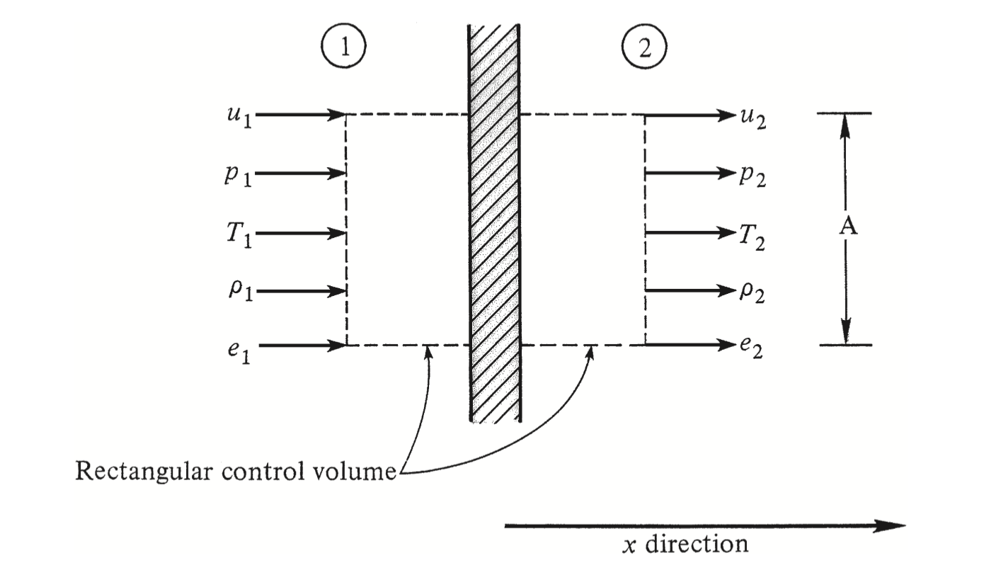
Consider a flow moving along the x x x
Figure 1: Anderson (1990)
Velocity: u u u Pressure: p p p Temperature: T T T Density: ρ \rho ρ Specific internal energy: e e e A A A A 1 = A 2 = A A_1 = A_2 = A A 1 = A 2 = A Derivation
1. Mass Conservation
The continuity equation, based on mass conservation, is:
− ∫ S ρ v ⋅ d s = ∂ ∂ t ∫ V ρ d V -\int_S \rho \mathbf{v} \cdot d\mathbf{s} = \frac{\partial}{\partial t} \int_V \rho dV − ∫ S ρ v ⋅ d s = ∂ t ∂ ∫ V ρ d V For steady flow (∂ ∂ t = 0 \frac{\partial}{\partial t} = 0 ∂ t ∂ = 0
∫ S ρ v ⋅ d s = 0 \int_S \rho \mathbf{v} \cdot d\mathbf{s} = 0 ∫ S ρ v ⋅ d s = 0 Along the x x x
− ρ 1 u 1 A + ρ 2 u 2 A = 0 -\rho_1 u_1 A + \rho_2 u_2 A = 0 − ρ 1 u 1 A + ρ 2 u 2 A = 0 Thus, ρ 1 u 1 = ρ 2 u 2 \rho_1 u_1 = \rho_2 u_2 ρ 1 u 1 = ρ 2 u 2
2. Momentum Equation
The momentum equation balances forces and momentum fluxes across the control volume, considering pressure and velocity changes.
The general form is:
∫ S ( ρ v ⋅ d s ) v + ∫ V ∂ ρ v ∂ t d V = − ∫ S p d s + ∫ S p f d V \int_S (\rho \mathbf{v} \cdot d\mathbf{s}) \mathbf{v} + \int_V \frac{\partial \mathbf{\rho v}}{\partial t} dV = -\int_S p d\mathbf{s} +\int_S p \mathbf{f} dV ∫ S ( ρ v ⋅ d s ) v + ∫ V ∂ t ∂ ρ v d V = − ∫ S p d s + ∫ S p f d V For steady flow with no body forces (f = 0 \mathbf{f}=\mathbf{0} f = 0
∫ S ( ρ v ⋅ d s ) v = − ∫ S p d s \int_S (\rho \mathbf{v} \cdot d\mathbf{s}) \mathbf{v} = -\int_S p d\mathbf{s} ∫ S ( ρ v ⋅ d s ) v = − ∫ S p d s Along x x x
− ρ 1 u 1 2 A + ρ 2 u 2 2 A = p 1 A − p 2 A -\rho_1 u_1^2 A + \rho_2 u_2^2 A = p_1 A - p_2 A − ρ 1 u 1 2 A + ρ 2 u 2 2 A = p 1 A − p 2 A The integrated form yields:
p 1 + ρ 1 u 1 2 = p 2 + ρ 2 u 2 2 p_1 + \rho_1 u_1^2 = p_2 + \rho_2 u_2^2 p 1 + ρ 1 u 1 2 = p 2 + ρ 2 u 2 2 3. Energy Equation
The energy equation accounts for internal energy, kinetic energy, heat, and work across the control volume.
The energy equation is:
∫ V q ˙ ρ d V − ∫ S p v ⋅ d S + ∫ V ρ ( f ⋅ v ) d V = ∫ V ∂ ∂ t ( ρ ( e + v 2 2 ) ) d V + ∫ S ρ ( e + v 2 2 ) v ⋅ d S \int_V {\dot{q} \rho dV} - \int_S {p\mathbf{v} \cdot d\mathbf{S}} + \int_V \rho (\mathbf{f}\cdot \mathbf{v})dV = \int_V {\frac{\partial}{\partial t} (\rho \left( e + \frac{v^2}{2} \right)) dV} + \int_S {\rho \left( e + \frac{v^2}{2} \right)} \mathbf{v}\cdot d\mathbf{S} ∫ V q ˙ ρ d V − ∫ S p v ⋅ d S + ∫ V ρ ( f ⋅ v ) d V = ∫ V ∂ t ∂ ( ρ ( e + 2 v 2 ) ) d V + ∫ S ρ ( e + 2 v 2 ) v ⋅ d S Here ∣ v ∣ = v |\mathbf{v}|=v ∣ v ∣ = v
For steady flow and zero body force, we get:
∫ V q ˙ ρ d V − ∫ S p v ⋅ d S = ∫ S ρ ( e + v 2 2 ) v ⋅ d S \int_V {\dot{q} \rho dV} - \int_S {p\mathbf{v} \cdot d\mathbf{S}} = \int_S {\rho \left( e + \frac{v^2}{2} \right)} \mathbf{v}\cdot d\mathbf{S} ∫ V q ˙ ρ d V − ∫ S p v ⋅ d S = ∫ S ρ ( e + 2 v 2 ) v ⋅ d S Integrating along x x x
− ρ 1 ( e 1 + u 1 2 2 ) u 1 A + ρ 2 ( e 2 + u 2 2 2 ) u 2 A = Q ˙ − ( − p 1 u 1 A + p 2 u 2 A ) -\rho_1 \left( e_1 + \frac{u_1^2}{2} \right) u_1 A + \rho_2 \left( e_2 + \frac{u_2^2}{2} \right) u_2 A = \dot{Q} - (-p_1 u_1 A + p_2 u_2 A) − ρ 1 ( e 1 + 2 u 1 2 ) u 1 A + ρ 2 ( e 2 + 2 u 2 2 ) u 2 A = Q ˙ − ( − p 1 u 1 A + p 2 u 2 A ) Here we define Q ˙ \dot{Q} Q ˙
Q ˙ A + p 1 u 1 + ρ 1 ( e 1 + u 1 2 2 ) u 1 = p 2 u 2 + ρ 2 ( e 2 + u 2 2 2 ) u 2 \frac{\dot{Q}}{A} + p_1 u_1 + \rho_1 \left( e_1 + \frac{u_1^2}{2} \right) u_1 = p_2 u_2 + \rho_2 \left( e_2 + \frac{u_2^2}{2} \right) u_2 A Q ˙ + p 1 u 1 + ρ 1 ( e 1 + 2 u 1 2 ) u 1 = p 2 u 2 + ρ 2 ( e 2 + 2 u 2 2 ) u 2 Dividing the left-hand side of equation by ρ 1 u 1 \rho_1 u_1 ρ 1 u 1 ρ 2 u 2 \rho_2 u_2 ρ 2 u 2 ρ 1 u 1 = ρ 2 u 2 \rho_1u_1=\rho_2u_2 ρ 1 u 1 = ρ 2 u 2 (3)
Q ˙ ρ 1 u 1 A + p 1 ρ 1 + e 1 + u 1 2 2 = p 2 ρ 2 + e 2 + u 2 2 2 \frac{\dot{Q}}{\rho_1 u_1 A} + \frac{p_1}{\rho_1} + e_1 + \frac{u_1^2}{2} = \frac{p_2}{\rho_2} + e_2 + \frac{u_2^2}{2} ρ 1 u 1 A Q ˙ + ρ 1 p 1 + e 1 + 2 u 1 2 = ρ 2 p 2 + e 2 + 2 u 2 2 Using enthalpy h = e + p ρ h = e + \frac{p}{\rho} h = e + ρ p m ˙ = ρ 1 u 1 A \dot{m} = \rho_1 u_1 A m ˙ = ρ 1 u 1 A
Q ˙ m ˙ + h 1 + v 1 2 2 = h 2 + v 2 2 2 \frac{\dot{Q}}{\dot{m}} + h_1 + \frac{v_1^2}{2} = h_2 + \frac{v_2^2}{2} m ˙ Q ˙ + h 1 + 2 v 1 2 = h 2 + 2 v 2 2 Here, the ratio Q ˙ m ˙ \frac{\dot{Q}}{\dot{m}} m ˙ Q ˙
Hence,
q + h 1 + v 1 2 2 = h 2 + v 2 2 2 q + h_1 + \frac{v_1^2}{2} = h_2 + \frac{v_2^2}{2} q + h 1 + 2 v 1 2 = h 2 + 2 v 2 2
Anderson, J. D. (1990). Modern compressible flow: with historical perspective. (None) .